V1 - Processing - timechart
timechart
- timechart {span="time", limit=N} <NAME = aggregate_function>, … by (groupByTerm)
The command timechart can be considered as a "matrix version" of aggregate. That is, within the interval of "time" and the limit number of N, do aggregate_functions according to (groupByTerm). f("@timestamp") has to be extracted before using the command timechart.
timechart-Table
The basic usage of timechart is given in the following example:
search
let source=f("@source"), size=f("__size__"), timestamp=f("@timestamp")
timechart {span="1h"} sourceCount=count() by source
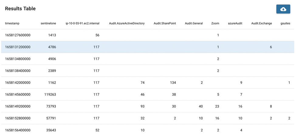
In the result, with the command timechart, a matrix is shown.
- Rows: time (with an interval of: span="time")
- Columns: source
To achieve the same goal, using aggregate would be like:
search
let source=f("@source"), size=f("__size__"), timestamp=f("@timestamp")
let Hour=strftime("%H:%M",timebucket("1h", timestamp))
aggregate sourceCount=count() by source, Hour
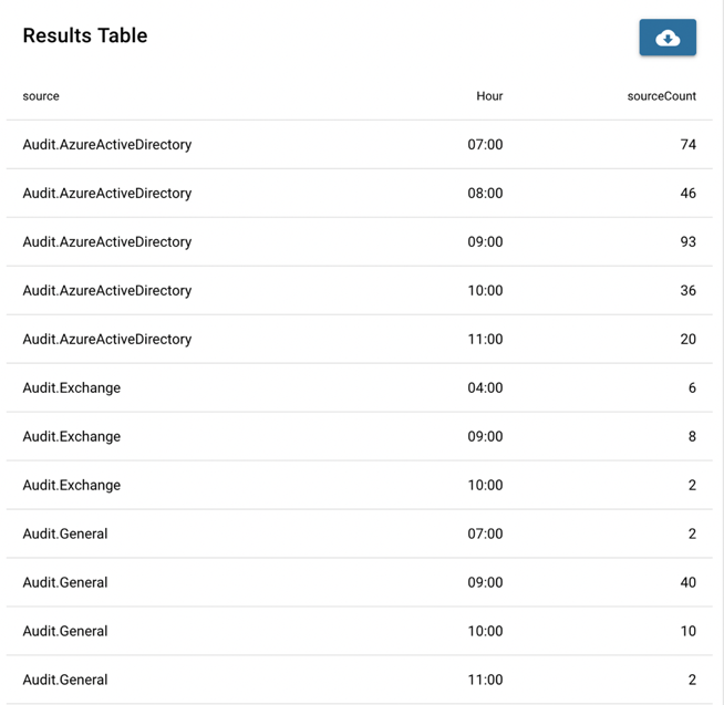
Comparing the result table of aggregate with the last one of timechart, one can find this table is kind of an "unfolded version" or "list version" of the last one. And in the result table of aggregate, if the count of a source in a one-hour interval is zero, this information cannot be shown. In a word, the timechart already contains the dimension of time internally, and displayed a two-dimensional result table.
timechart-Histogram
Another important usage of timechart is to present histogram with time as X axis, i.e. the time series of a variable.
Example:
function aws_Region()
    search {from="-7d@d", to="@d"} sContent("@event_type","@cloudtrail")
    let {awsRegion} =f("@cloudtrail")
    aggregate count_Region=count() by awsRegion
    sort count_Region
end
function aws_Region_timechart()
    search {from="-7d@d", to="@d"} sContent("@event_type","@cloudtrail")
    let {awsRegion} =f("@cloudtrail")
    let timestamp=f("@timestamp")
    timechart {span="1h"} count_Region_timechart=count() by awsRegion
end
stream aws_Region=aws_Region()
stream aws_Region_timechart=aws_Region_timechart()
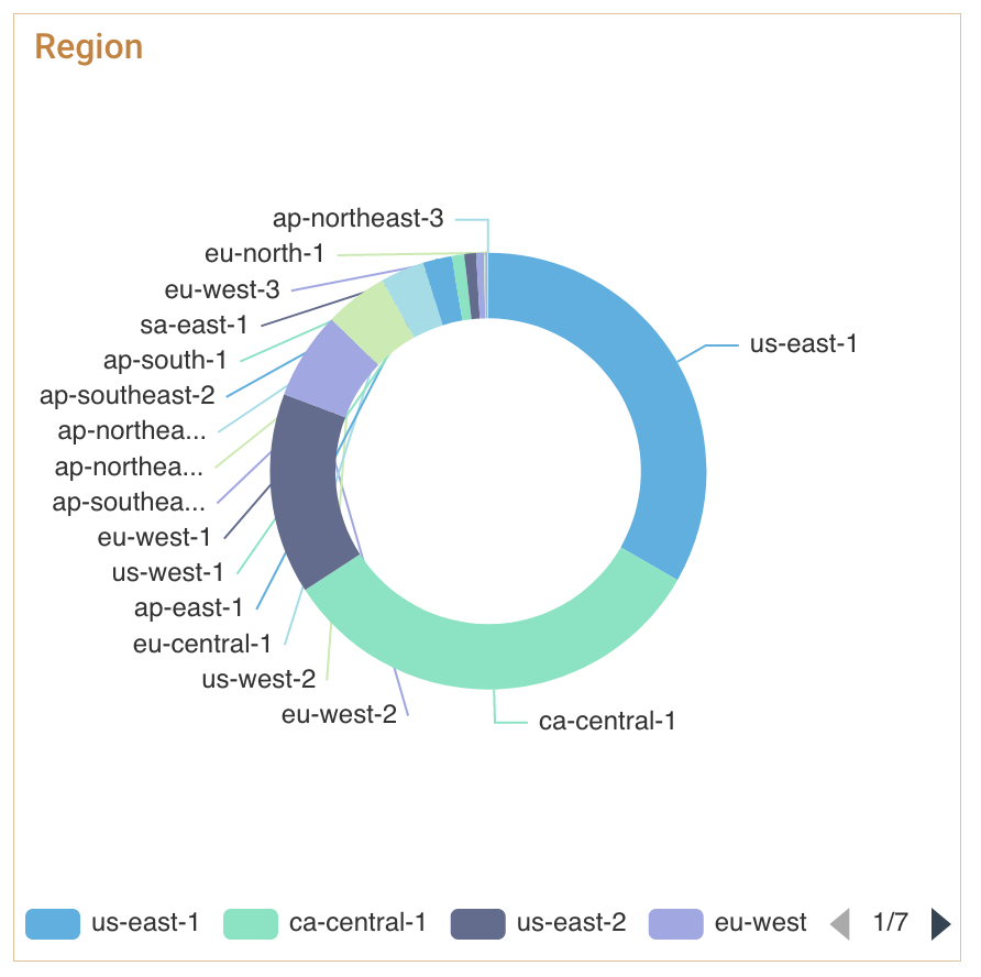
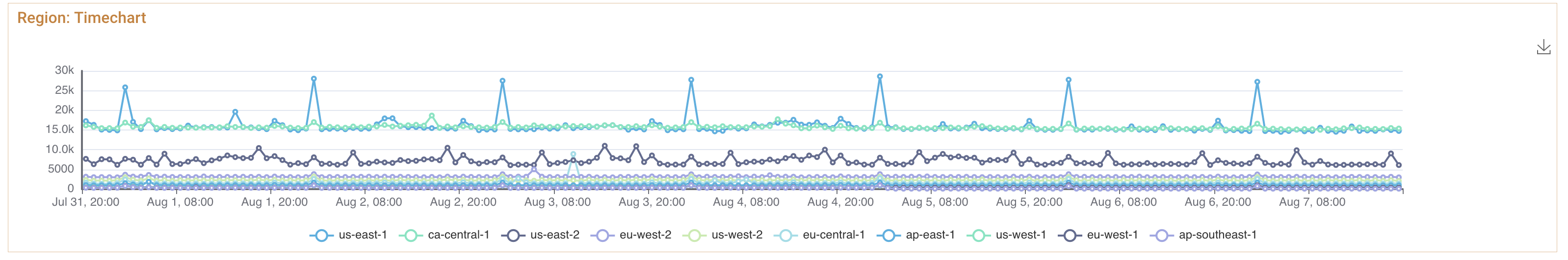
In the example above, the basic statistics (illustrated by Pie Chart) of aws_Region is achieved by aggregate("function aws_Region()"). On the other hand, how does the number of each aws_Region vary with time (illustrated by Histogram) is given by timechart ("function aws_Region_timechart()"). Therefore, timechart is an fundemental tool in creating FPL reports.